Tree Ensembles: Random Forests and Gradient Boosting

Not every prediction problem is an image or a sequence. Most epidemiological data is tabular — rows of patients or places, columns of mixed-type features — and for that data the best off-the-shelf models are usually not neural networks but ensembles of decision trees. A single tree is weak and unstable; combine hundreds of them, by averaging (random forests) or by sequentially correcting their mistakes (gradient boosting), and you get models that are accurate, robust to messy features, need little tuning, and report which variables matter — which is why they dominate tabular-data competitions and clinical risk modeling alike.

The decision tree#

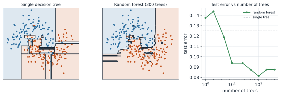
A decision tree predicts by asking a sequence of yes/no questions about the features — “age > 65?”, “CRP > 40?” — each splitting the data, until a leaf assigns a prediction. Training grows the tree greedily: at each node it searches every feature and threshold for the split that most purifies the two resulting groups, measured by impurity — the Gini index or entropy for classification, variance for regression — and repeats until the leaves are pure or a stopping rule fires. The result is an axis-aligned partition of feature space into boxes, each with its own prediction, and trees have real virtues: they handle numeric and categorical features together, need no scaling, capture interactions automatically, and are readable. Their fatal flaw is variance: a fully grown tree fits the training data almost perfectly and its jagged boundary (left of the figure) changes wildly if the data shift slightly — a textbook overfitter.

Bagging and random forests#

The fix is to average many trees so their errors cancel. Bagging (bootstrap aggregating) trains each tree on a different bootstrap resample of the data and averages their predictions; because averaging reduces variance, the ensemble is far more stable than any single tree. A random forest adds one more twist that makes it work spectacularly: at each split, each tree may consider only a random subset of the features. This decorrelates the trees — they cannot all seize on the same one dominant predictor — and averaging decorrelated trees cuts variance much more than averaging near-identical ones. The middle panel of the figure shows the payoff: hundreds of jagged trees average into a smooth, sensible boundary, and the right panel shows test error falling and flattening as trees are added, well below the single tree’s. A free bonus is the out-of-bag error estimate: each tree can be validated on the samples its bootstrap left out, giving a built-in cross-validation-like score at no extra cost.

Boosting#

Boosting takes the opposite tack: instead of many independent trees averaged in parallel, it builds trees sequentially, each one correcting the errors of those before it. Gradient boosting makes this precise — it fits each new tree to the negative gradient of the loss (for squared error, simply the residuals) of the current ensemble, then adds it in, scaled by a small learning rate: $$F_{m}(x) = F_{m-1}(x) + \eta\, h_m(x), \qquad h_m \approx -\frac{\partial \mathcal{L}}{\partial F_{m-1}}.$$ Each tree is a small step down the loss’s gradient in function space, so a boosted ensemble of shallow trees becomes a highly accurate model. The modern implementations — XGBoost, LightGBM, and scikit-learn’s histogram gradient boosting — are the tools that win most tabular competitions and power many production risk models. Boosting can overfit if run too long, so the number of trees, the learning rate, and the tree depth are tuned by cross-validation with early stopping — a smaller $\eta$ with more trees usually generalizes best.

Feature importance and interpretability#

A practical reason to reach for tree ensembles is that they say which features drove the prediction. The simplest measure is impurity importance — how much each feature reduced impurity across all splits — but it is biased toward high-cardinality features, so permutation importance (how much accuracy drops when a feature’s values are shuffled) is more trustworthy, and SHAP values give per-prediction attributions grounded in game theory. This interpretability matters in health settings, where a model that flags a patient as high-risk must be able to say why before a clinician will act on it — though importance is about association in the model, not causation, and should not be read as a causal effect.

A worked example#

Consider a node splitting $100$ patients, $50$ with a severe outcome and $50$ without, on “age > 65”. Suppose the split sends $40$ patients left ($10$ severe, $30$ not) and $60$ right ($40$ severe, $20$ not). The Gini impurity of a group with severe fraction $p$ is $2p(1-p)$; the parent is $2(0.5)(0.5)=0.5$. The left child has $p=0.25$, impurity $2(0.25)(0.75)=0.375$; the right has $p\approx0.67$, impurity $2(0.67)(0.33)=0.444$. The weighted child impurity is $0.4(0.375)+0.6(0.444)=0.416$, so this split lowers impurity from $0.5$ to $0.416$ — a Gini gain of $0.084$, and the tree picks whichever feature and threshold maximize that gain.

In code#

Python#

A random forest and a gradient-boosting model both train in a couple of lines and report accuracy, calibrated probabilities, and feature importances:

import numpy as np
from sklearn.datasets import make_classification
from sklearn.model_selection import train_test_split
from sklearn.ensemble import RandomForestClassifier, HistGradientBoostingClassifier
from sklearn.metrics import roc_auc_score

# a synthetic "severe outcome" dataset: 8 features, 4 truly informative
X, y = make_classification(n_samples=2000, n_features=8, n_informative=4,
                           n_redundant=2, random_state=0)
Xtr, Xte, ytr, yte = train_test_split(X, y, test_size=0.3, random_state=0)

rf = RandomForestClassifier(n_estimators=300, random_state=0).fit(Xtr, ytr)
gb = HistGradientBoostingClassifier(random_state=0).fit(Xtr, ytr)
for name, model in [("random forest", rf), ("gradient boosting", gb)]:
    auc = roc_auc_score(yte, model.predict_proba(Xte)[:, 1])
    print(f"{name:18s} test AUC {auc:.3f}")

imp = rf.feature_importances_                       # which features mattered
top = np.argsort(imp)[::-1][:4]
print("top features (index: importance):",
      [(int(i), round(float(imp[i]), 2)) for i in top])

random forest      test AUC 0.973
gradient boosting  test AUC 0.967
top features (index: importance): [(5, 0.19), (1, 0.17), (0, 0.16), (7, 0.15)]

The gradient-boosting library used in practice is XGBoost, and SHAP (TreeExplainer) attributes each prediction to its features — both run here on the same data:

import xgboost as xgb
import shap

xgbm = xgb.XGBClassifier(n_estimators=300, learning_rate=0.05, max_depth=4,
                         random_state=0).fit(Xtr, ytr)
print(f"XGBoost test AUC {roc_auc_score(yte, xgbm.predict_proba(Xte)[:, 1]):.3f}")

sv = shap.TreeExplainer(xgbm).shap_values(Xte)      # exact, fast SHAP for trees
mean_abs = np.abs(sv).mean(0)                         # global feature importance
order = np.argsort(mean_abs)[::-1][:4]
print("top features by mean |SHAP|:",
      [(int(i), round(float(mean_abs[i]), 2)) for i in order])

XGBoost test AUC 0.963
top features by mean |SHAP|: [(5, 1.1), (1, 0.82), (7, 0.78), (0, 0.75)]

R#

# ranger for fast random forests; xgboost / lightgbm for boosting.
library(ranger)
rf <- ranger(outcome ~ ., data = train, num.trees = 500, importance = "permutation")
rf$prediction.error                 # out-of-bag error
sort(importance(rf), decreasing = TRUE)[1:5]

Julia#

# MLJ wraps DecisionTree.jl (forests) and EvoTrees.jl / XGBoost.jl (boosting).
using MLJ
Forest = @load RandomForestClassifier pkg=DecisionTree
mach = machine(Forest(n_trees = 500), X, y) |> fit!
feature_importances(mach)

Why it matters#

For the tabular prediction tasks that fill applied epidemiology — a clinical risk score from electronic health records, a triage model from vitals and labs, a hotspot predictor from surveillance and covariate tables — tree ensembles are usually the right first (and often last) model. They tolerate missing values and mixed feature types, need almost no preprocessing, resist overfitting when tuned, and, crucially, expose which features drive their predictions, which is what lets a clinician or public-health official trust and interrogate them. Reach for a neural network when the data are images, sequences, or graphs with structure to exploit; reach for a tree ensemble when the data are a table — and either way, hold the model to the same validation discipline, because a boosted forest can memorize noise as eagerly as any network.

Related#

• Overfitting, Regularization, and Cross-Validation
• Neural Networks and the Multilayer Perceptron
• Sampling Distributions
• Logistic Regression
• Diagnostic Testing and Screening
• Proper Scoring Rules
• Quantitative Methods