Type M and Type S Errors
Classical power analysis asks a single question: what is the chance of getting a statistically significant result? But a significant result is not automatically a good result. When a study is underpowered, the estimates that happen to clear the significance threshold are a biased, selected sample — they are systematically too big, and a worrying fraction of them have the wrong sign. Gelman and Carlin (2014) call the accounting of these two failure modes design analysis, and they name the errors after the part of the estimate they corrupt:
- a Type M (“magnitude”) error — the exaggeration ratio — is how many times larger a significant estimate is than the true effect, on average;
- a Type S (“sign”) error is the probability that a significant estimate has the opposite sign from the true effect.
These are the errors that survive publication. A study reports “, effect ”, the true effect is , and nobody notices that the design guaranteed a fivefold overstatement.
The one number that drives everything#
Fix a hypothesized true effect and the standard error that a proposed design would give (from its sample size, outcome variance, and analysis). Everything below depends only on their ratio,
the true effect measured in standard errors. A two-sided test at level rejects when the estimate exceeds in absolute value, where . Treating the estimate as normal, , the three design quantities are
where and are the standard normal CDF and density. The two terms in the power (1) are the chance of a significant estimate with the correct sign and with the wrong sign; Type S (2) is just the wrong-sign share. Type M (3) is the mean absolute significant estimate divided by — the conditional expectation worked out for the truncated normal.
Gelman and Carlin’s original retrodesign computes Type M by simulation (draw many , keep the significant ones, average ).
The closed forms above give the same answer without a random seed and use a normal reference; swap for their counterparts when the design’s degrees of freedom are small.
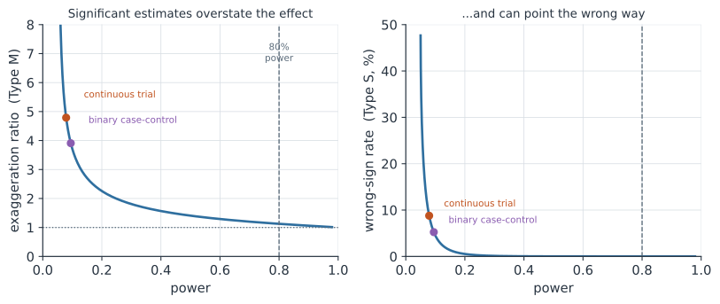
The behavior is stark (Figure 1). As power drops toward , the exaggeration ratio diverges and the sign error rate climbs toward one-half — a barely-significant study is close to a coin flip on direction and inflates whatever it does find. At the conventional 80% power target, Type M is about and Type S is essentially zero, which is exactly why design analysis mostly reassures well-powered studies and indicts underpowered ones.
Worked example 1 — a continuous outcome#
A small trial estimates how much a monoclonal antibody lowers peak viral load, measured in copies/mL. Suppose the true reduction is a modest , and the trial’s size and outcome variance yield a standard error . Then : power is only about , so the study is severely underpowered. Conditional on reaching significance, the estimate overstates the true effect by a factor of roughly (a reported reduction near for a true ), and about of significant estimates would claim the antibody raises viral load.
Worked example 2 — a binary outcome#
For a binary outcome the effect usually lives on the log-odds-ratio scale, and the standard error comes straight from the cell counts of the table via Woolf’s formula, . Consider a small case-control study of a suspected risk factor with
| exposed | unexposed | |
|---|---|---|
| cases | 15 | 85 |
| controls | 12 | 88 |
giving an odds ratio of , so and , hence . Power is about ; a significant odds ratio would exaggerate the true association nearly fourfold on the log scale, and about of significant results would report a protective factor as harmful (or vice versa). The lesson generalizes: sparse tables make large, push down, and turn every “significant” odds ratio into a likely overstatement.
In code#
A single design_analysis(effect, se, alpha) returns power, the Type S rate, and the Type M exaggeration ratio, then we feed it both examples.
R#
design_analysis <- function(effect, se, alpha = 0.05) {
  d  <- abs(effect) / se
  zc <- qnorm(1 - alpha / 2)
  p_hi  <- pnorm(d - zc)           # significant, correct sign
  p_lo  <- pnorm(-zc - d)          # significant, wrong sign
  power <- p_hi + p_lo
  type_m <- (d * (p_hi - p_lo) + dnorm(zc - d) + dnorm(zc + d)) / (d * power)
  list(power = power, type_s = p_lo / power, type_m = type_m)
}

# Example 1: continuous outcome (log10 viral load reduction)
design_analysis(effect = 0.30, se = 0.60)

# Example 2: binary outcome, SE from the 2x2 table (Woolf's formula)
a <- 15; b <- 85; c <- 12; d <- 88
logor <- log((a * d) / (b * c))
se    <- sqrt(1/a + 1/b + 1/c + 1/d)
design_analysis(effect = logor, se = se)
Python#
from math import log, sqrt
from scipy.stats import norm

def design_analysis(effect, se, alpha=0.05):
    d = abs(effect) / se
    zc = norm.ppf(1 - alpha / 2)
    p_hi = norm.cdf(d - zc)           # significant, correct sign
    p_lo = norm.cdf(-zc - d)          # significant, wrong sign
    power = p_hi + p_lo
    type_m = (d * (p_hi - p_lo) + norm.pdf(zc - d) + norm.pdf(zc + d)) / (d * power)
    return {"power": power, "type_s": p_lo / power, "type_m": type_m}

def show(label, r):
    print(f"{label:>12}: power={r['power']:.3f}  "
          f"Type S={r['type_s']*100:5.2f}%  Type M={r['type_m']:.2f}")

# Example 1: continuous outcome (log10 viral load reduction)
show("continuous", design_analysis(0.30, 0.60))

# Example 2: binary outcome, SE from the 2x2 table (Woolf's formula)
a, b, c, d = 15, 85, 12, 88
logor = log((a * d) / (b * c))
se = sqrt(1/a + 1/b + 1/c + 1/d)
show("binary", design_analysis(logor, se))
  continuous: power=0.079  Type S= 8.78%  Type M=4.79
      binary: power=0.095  Type S= 5.20%  Type M=3.90
Julia#
using Distributions

function design_analysis(effect, se; alpha = 0.05)
    d  = abs(effect) / se
    zc = quantile(Normal(), 1 - alpha / 2)
    p_hi  = cdf(Normal(), d - zc)        # significant, correct sign
    p_lo  = cdf(Normal(), -zc - d)       # significant, wrong sign
    power = p_hi + p_lo
    type_m = (d * (p_hi - p_lo) + pdf(Normal(), zc - d) +
              pdf(Normal(), zc + d)) / (d * power)
    (power = power, type_s = p_lo / power, type_m = type_m)
end

# Example 1: continuous outcome
design_analysis(0.30, 0.60)

# Example 2: binary outcome, SE from the 2x2 table (Woolf's formula)
a, b, c, d = 15, 85, 12, 88
logor = log((a * d) / (b * c))
se = sqrt(1/a + 1/b + 1/c + 1/d)
design_analysis(logor, se)
Putting it together: a complete binary-outcome workflow#
Design analysis earns its keep as the last step of a workflow that begins before any data are collected. Here is the whole arc for a binary outcome, from the a-priori sample size to the retrospective check that keeps a lucky result honest.
A trial of a prophylactic aims to cut a post-operative infection risk of by a modest but genuinely worthwhile amount — an odds ratio of . A standard two-sided calculation at power says the trial needs about patients per arm, in all. Accrual is slow, though, and the trial closes with only per arm — a shortfall of nearly three-quarters of the planned sample. The analysis then turns up exactly the kind of result that feels like a reward for the struggle: infections on treatment versus on control, an odds ratio of with . Before celebrating, run the design analysis using the study’s own standard error and the modest effect the trial was actually built to detect. Even granting that the drug truly helps at OR , this study had only about power, so a significant estimate exaggerates the log-odds effect by roughly on average and would land near an odds ratio of . The direction is trustworthy (Type S well under ), but the eye-catching is almost certainly an inflated draw, not evidence that the effect is enormous.
import math

# Step 1 — a-priori sample size to detect the smallest effect worth finding
def n_per_arm_logor(p0, odds_ratio, alpha=0.05, power=0.80):
    odds0 = p0 / (1 - p0)
    p1 = odds_ratio * odds0 / (1 + odds_ratio * odds0)
    var_factor = 1/p1 + 1/(1 - p1) + 1/p0 + 1/(1 - p0)   # SE(logOR)^2 = factor / n
    se_target = abs(math.log(odds_ratio)) / (norm.ppf(1 - alpha/2) + norm.ppf(power))
    return math.ceil(var_factor / se_target**2)

p0, or_design = 0.30, 0.65                      # control risk; smallest worthwhile effect
n_req = n_per_arm_logor(p0, or_design)
print(f"Step 1  design: OR={or_design} at 80% power needs {n_req}/arm ({2*n_req} total)")

# Step 2 — reality: accrual falls short
n_obs = 120
print(f"Step 2  enrolled {n_obs}/arm ({2*n_obs} total): a {1 - n_obs/n_req:.0%} shortfall")

# Step 3 — the tempting result: a big, significant odds ratio
a, b = 12, n_obs - 12          # treated:  infected, not
c, d = 33, n_obs - 33          # control:  infected, not
or_obs = (a * d) / (b * c)
se_obs = math.sqrt(1/a + 1/b + 1/c + 1/d)
z = math.log(or_obs) / se_obs
print(f"Step 3  observed OR={or_obs:.2f}  (SE={se_obs:.2f}, z={z:.2f}, "
      f"p={2*norm.cdf(-abs(z)):.1e}) — significant!")

# Step 4 — retrospective design analysis at the study's own SE,
#          assuming the truth is the modest effect the trial was built for
r = design_analysis(math.log(or_design), se_obs)
avg_sig = math.exp(-r["type_m"] * abs(math.log(or_design)))
print(f"Step 4  if the truth is OR={or_design}: power={r['power']:.2f}, "
      f"Type S={r['type_s']*100:.1f}%, Type M={r['type_m']:.1f}")
print(f"        a significant study averages OR {avg_sig:.2f}; "
      f"the observed {or_obs:.2f} is an inflated draw")
Step 1  design: OR=0.65 at 80% power needs 450/arm (900 total)
Step 2  enrolled 120/arm (240 total): a 73% shortfall
Step 3  observed OR=0.29  (SE=0.37, z=-3.35, p=8.1e-04) — significant!
Step 4  if the truth is OR=0.65: power=0.22, Type S=0.4%, Type M=2.2
        a significant study averages OR 0.40; the observed 0.29 is an inflated draw
The takeaway is not that the treatment fails — the sign is reliable and it may well help — but that the magnitude on display is untrustworthy, and the honest point estimate is far closer to the modest effect the trial set out to detect than to the dramatic one it happened to report.
Why it matters#
Design analysis reframes what a “significant” finding is worth in the very regime where infectious-disease work often operates: small trials, rare events, sparse contingency tables, subgroup analyses, and pilot studies. In all of these the standard error is large, is small, and statistical significance becomes a filter that admits only the luckiest, most exaggerated estimates — a mechanism behind the winner’s curse and much of the replication crisis. The practical move is to run (1)–(3) before collecting data, using a defensible guess for the true effect: if the design implies a Type M of 4 or a Type S above a few percent, a significant result will not mean what you want it to, and the fix is a bigger study, a better outcome, or a more honest confidence interval rather than a -value.