The 2001 UK Foot-and-Mouth Epidemic: Spatial Spread and Control
The 2001 foot-and-mouth epidemic swept through the United Kingdom’s livestock, and because every farm’s location and stock were recorded, it left behind an unusually fine-grained picture of an outbreak spreading between fixed points on a map. Keeling et al., 2001, Science turned that picture into an individual farm-based stochastic model, and used it to read the epidemic’s spatial dynamics and to weigh the control options while the crisis was still unfolding. It is a landmark case study because it shows the whole chain at once — detection, modeling, and response — and how the geometry of spread decides which control works.
Why a well-mixed model fails here#
Cases of foot-and-mouth did not appear at random across the country; they clustered, with new infections landing close to existing ones. A standard mass-action SIR model assumes every host mixes with every other equally, so it cannot represent a disease whose next case is almost always a near neighbor of the last. The spatial clustering is the signal, not noise, and capturing it means abandoning homogeneous mixing for a model that knows where each farm sits. This is the same move that motivates spatiotemporal models and spatial diffusion: once transmission depends on distance, the map becomes part of the state.
The transmission kernel: local spread with long-range sparks#
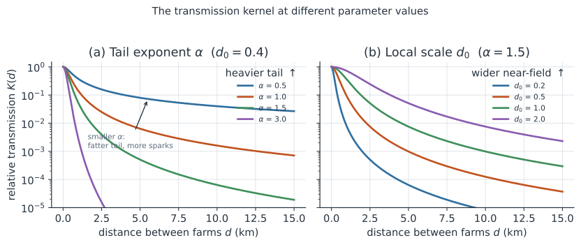
The engine of a spatial model is the transmission kernel , the relative rate at which infection passes between two farms a distance apart. For foot-and-mouth the kernel is fat-tailed: a high probability of short-range spread to immediate neighbors, combined with a long tail of occasional long-range “sparks” that seed a fresh cluster far away. A convenient illustrative form is with a local scale and a tail exponent that controls how heavy the tail is. Varying those two parameters traces the whole family: a smaller fattens the tail so long-range sparks become more likely, while a larger widens the near-field over which spread is almost certain.
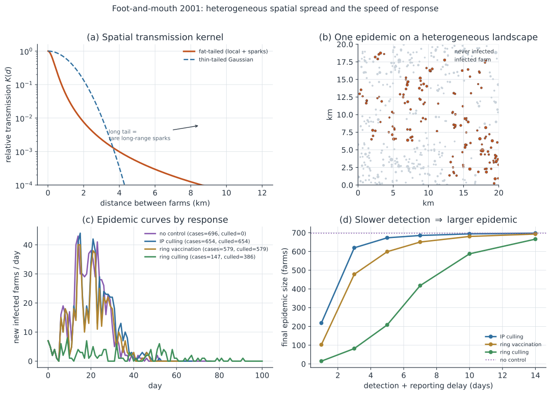
The contrast in the main figure’s panel (a) is the whole point: a thin-tailed Gaussian kernel falls off so fast that long jumps essentially never happen, whereas the fat-tailed kernel keeps a small but real chance of a distant spark. Those sparks matter because they are what let an epidemic escape a local firebreak, and they are the spatial cousin of the heavy tails that drive superspreading and jumps across a contact network.
A farm-based stochastic model#
The model treats the farm, not the animal, as the unit, classifying each holding as susceptible, incubating, infectious, or culled. Farms are not interchangeable: a holding’s susceptibility and infectiousness both scale with its size and species composition, so a large mixed farm is both a bigger target and a bigger source than a small one. Writing for the susceptibility of farm and for the infectiousness of an infectious farm , the daily force of infection on a susceptible farm is a kernel-weighted sum over every infectious farm, and is the probability that farm is infected that day. Newly infected farms incubate for a latent period before becoming infectious, and the whole process is run forward stochastically one day at a time, so chance and geometry together produce the irregular, clustered spread seen in panel (b). Because transmission is a chance event on a finite landscape, the model is a spatial version of the stochastic epidemics idea: the same can give a small contained cluster or a national epidemic depending on where the early sparks land.
Control as a spatial strategy#
Once a farm is detected — after a detection-and-reporting delay that is itself part of the response — the model can apply a control measure to it and its surroundings. Three strategies span the options that were debated in 2001.
- Infected-premises (IP) culling removes only the reported farm once it is detected. It is the narrowest response, and it lags the infection by the reporting delay.
- Ring (neighborhood or contiguous-premises) culling removes the detected farm together with every farm inside a radius, susceptible or not, pre-emptively cutting the local kernel. It prevents cases at the cost of culling healthy farms.
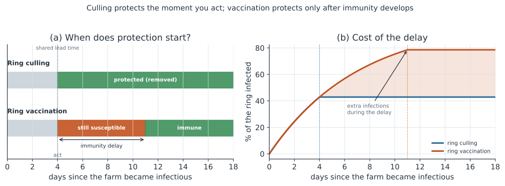
- Ring vaccination immunizes susceptible farms inside the radius instead of killing them, but protection arrives only after a decision-to-immunity delay, during which those farms can still be infected.
The choice is not abstract: it decides how the response meets the kernel in space and time. The responses differ above all in timing: culling protects the moment it is applied, whereas vaccination leaves a ring susceptible through the delay while immunity develops, so cases keep accruing there until protection takes hold.
Speed and targeting: the response trade-off#
The model’s central lesson is that speed and spatial targeting dominate. Panel (c) shows that infected-premises culling alone barely bends the epidemic, because it always trails the reporting delay while the fat tail keeps seeding new clusters, whereas ring culling flattens the curve by cutting the kernel ahead of the spread. Ring vaccination lands in between, and it loses to ring culling for a specific reason Keeling et al. emphasized: the delay between the decision to vaccinate and the onset of immunity lets infection race through the ring before protection takes hold, so vaccination yields a larger epidemic than tightly focused neighborhood culling. Panel (d) turns speed into the x-axis directly — as the detection-and-reporting delay grows, every control’s final epidemic size climbs toward the no-control ceiling, and the advantage of ring culling is largest exactly when the response is fast. This is the “hit hard, hit early” tenet familiar from livestock and human epidemics, and shown for wildlife disease by Bozzuto et al., 2020, Proc. R. Soc. B: the window for intervention shrinks rapidly if detection is late, so a delayed response can negate the benefit of acting at all. Two costs sit behind the headline: ring culling buys fewer cases by culling many healthy farms pre-emptively, which is an ethical and economic burden, not a free win. Note too that in this outbreak the affected unit is a farm of animals, not a person — a reminder that the “person” axis of a case definition generalizes to whatever host the outbreak is in.
A worked example#
Running the illustrative model below on a synthetic 400-farm landscape (no real data) reproduces the ordering seen in the figure. With a detection delay of four days, no control infects almost every farm, infected-premises culling shaves only a little off that total, ring vaccination does better, and ring culling ends the epidemic with a small fraction of farms infected — while culling many healthy farms to do so. Sweeping the detection delay for ring culling shows the interplay directly: acting two days after a farm becomes infectious contains the outbreak to a handful of farms, but waiting ten days lets it grow by more than an order of magnitude. Detection speed, response strategy, and the spatial model are one system, not three separate concerns.
In code#
We build the fat-tailed kernel on a heterogeneous farm landscape, run the daily stochastic model, and compare the control strategies. The R and Julia versions mirror the Python.
R#
set.seed(2001)
N <- 400; SIDE <- 15; D0 <- 0.4; BETA <- 0.65
LATENT <- 5L; VACC_DELAY <- 7L

xy   <- matrix(runif(N * 2, 0, SIDE), N, 2)
size <- rlnorm(N, 0, 0.7)                         # farm-size heterogeneity
d    <- as.matrix(dist(xy))
K    <- (1 + (d / D0)^2)^(-1.5)                   # fat-tailed spatial kernel
diag(K) <- 0

epidemic <- function(strategy = "none", detect_delay = 4, ring = 1.5,
                     days = 160) {
  st <- integer(N); lat <- rep(-1L, N); ic <- rep(-1L, N)
  vp <- logical(N); vc <- rep(-1L, N); ever <- logical(N); culled <- 0L
  seeds <- sample(N, 3); st[seeds] <- 2L; ic[seeds] <- 0L; ever[seeds] <- TRUE
  for (day in seq_len(days)) {
    inf <- which(st == 2L)
    if (length(inf)) {
      foi <- BETA * size * (K[, inf, drop = FALSE] %*% size[inf])
      new <- st == 0L & runif(N) < 1 - exp(-foi)
      st[new] <- 1L; lat[new] <- 0L; ever[new] <- TRUE; vp[new] <- FALSE
    }
    for (s in which(st == 2L & ic == detect_delay)) {
      if (strategy %in% c("ip", "ring", "vacc") && st[s] != 3L) {
        st[s] <- 3L; culled <- culled + 1L
      }
      if (strategy == "ring") {
        near <- which(d[s, ] <= ring & st != 3L)
        culled <- culled + length(near); st[near] <- 3L
      } else if (strategy == "vacc") {
        vac <- which(d[s, ] <= ring & st == 0L & !vp)
        vp[vac] <- TRUE; vc[vac] <- 0L
      }
    }
    mat <- vp & vc >= VACC_DELAY; st[mat] <- 4L; vp[mat] <- FALSE
    if (strategy == "none") st[st == 2L & ic >= 14L] <- 3L
    prog <- st == 1L & lat >= LATENT; st[prog] <- 2L; ic[prog] <- 0L
    lat[st == 1L] <- lat[st == 1L] + 1L
    ic[st == 2L]  <- ic[st == 2L] + 1L
    vc[vp] <- vc[vp] + 1L
    if (!any(st == 1L) && !any(st == 2L)) break
  }
  c(cases = sum(ever), culled = culled)
}

for (s in c("none", "ip", "vacc", "ring")) print(epidemic(s))
Python#
import numpy as np

rng = np.random.default_rng(2001)
N, SIDE, D0, BETA = 400, 15.0, 0.4, 0.65
LATENT, VACC_DELAY = 5, 7

xy = rng.uniform(0, SIDE, size=(N, 2))
size = rng.lognormal(0.0, 0.7, size=N)          # farm-size heterogeneity
d = np.sqrt(((xy[:, None] - xy[None, :]) ** 2).sum(-1))
K = (1.0 + (d / D0) ** 2) ** (-1.5)             # fat-tailed spatial kernel
np.fill_diagonal(K, 0.0)

def epidemic(strategy="none", detect_delay=4, ring=1.5, days=160, seed=0):
    r = np.random.default_rng(seed)
    st = np.zeros(N, int); lat = np.full(N, -1); ic = np.full(N, -1)
    vp = np.zeros(N, bool); vc = np.full(N, -1); ever = np.zeros(N, bool)
    culled = 0
    seeds = r.choice(N, 3, replace=False); st[seeds] = 2; ic[seeds] = 0
    ever[seeds] = True
    for _ in range(days):
        I = np.where(st == 2)[0]
        if I.size:                               # kernel-weighted force of infection
            foi = BETA * size * (K[:, I] @ size[I])
            new = (st == 0) & (r.random(N) < 1 - np.exp(-foi))
            st[new] = 1; lat[new] = 0; ever[new] = True; vp[new] = False
        for s in np.where((st == 2) & (ic == detect_delay))[0]:
            if strategy in ("ip", "ring", "vacc") and st[s] != 3:
                st[s] = 3; culled += 1
            if strategy == "ring":               # cull the neighbourhood
                near = np.where((d[s] <= ring) & (st != 3))[0]
                culled += near.size; st[near] = 3
            elif strategy == "vacc":             # vaccinate susceptibles in ring
                vac = np.where((d[s] <= ring) & (st == 0) & ~vp)[0]
                vp[vac] = True; vc[vac] = 0
        mat = vp & (vc >= VACC_DELAY); st[mat] = 4; vp[mat] = False   # immunity
        if strategy == "none":
            st[(st == 2) & (ic >= 14)] = 3
        prog = (st == 1) & (lat >= LATENT); st[prog] = 2; ic[prog] = 0
        lat[st == 1] += 1; ic[st == 2] += 1; vc[vp] += 1
        if not ((st == 1).any() or (st == 2).any()):
            break
    return int(ever.sum()), culled

print(f"{'strategy':16s}{'cases':>7s}{'culled':>8s}")
for s, lab in [("none", "no control"), ("ip", "IP culling"),
               ("vacc", "ring vaccination"), ("ring", "ring culling")]:
    c, k = epidemic(s, seed=7)
    print(f"{lab:16s}{c:7d}{k:8d}")
delays = {dl: epidemic("ring", detect_delay=dl, seed=7)[0] for dl in (2, 6, 10)}
print("ring cull, cases by detection delay:",
      "  ".join(f"d={k}->{v}" for k, v in delays.items()))
strategy          cases  culled
no control          399       0
IP culling          358     358
ring vaccination    269     269
ring culling         65     183
ring cull, cases by detection delay: d=2->5  d=6->117  d=10->289
Julia#
using Random, LinearAlgebra
Random.seed!(2001)
const N, SIDE, D0, BETA = 400, 15.0, 0.4, 0.65
const LATENT, VACC_DELAY = 5, 7

xy   = rand(N, 2) .* SIDE
size = exp.(randn(N) .* 0.7)                      # farm-size heterogeneity
d    = [sqrt(sum((xy[i, :] .- xy[j, :]).^2)) for i in 1:N, j in 1:N]
K    = (1 .+ (d ./ D0).^2).^(-1.5)                # fat-tailed spatial kernel
K[diagind(K)] .= 0.0

function epidemic(strategy="none"; detect_delay=4, ring=1.5, days=160)
    st = zeros(Int, N); lat = fill(-1, N); ic = fill(-1, N)
    vp = falses(N); vc = fill(-1, N); ever = falses(N); culled = 0
    seeds = randperm(N)[1:3]; st[seeds] .= 2; ic[seeds] .= 0; ever[seeds] .= true
    for _ in 1:days
        inf = findall(==(2), st)
        if !isempty(inf)
            foi = BETA .* size .* (K[:, inf] * size[inf])
            new = (st .== 0) .& (rand(N) .< 1 .- exp.(-foi))
            st[new] .= 1; lat[new] .= 0; ever[new] .= true; vp[new] .= false
        end
        for s in findall(i -> st[i] == 2 && ic[i] == detect_delay, 1:N)
            if strategy in ("ip", "ring", "vacc") && st[s] != 3
                st[s] = 3; culled += 1
            end
            if strategy == "ring"
                near = findall(j -> d[s, j] <= ring && st[j] != 3, 1:N)
                culled += length(near); st[near] .= 3
            elseif strategy == "vacc"
                vac = findall(j -> d[s, j] <= ring && st[j] == 0 && !vp[j], 1:N)
                vp[vac] .= true; vc[vac] .= 0
            end
        end
        mat = vp .& (vc .>= VACC_DELAY); st[mat] .= 4; vp[mat] .= false
        strategy == "none" && (st[(st .== 2) .& (ic .>= 14)] .= 3)
        prog = (st .== 1) .& (lat .>= LATENT); st[prog] .= 2; ic[prog] .= 0
        lat[st .== 1] .+= 1; ic[st .== 2] .+= 1; vc[vp] .+= 1
        (any(st .== 1) || any(st .== 2)) || break
    end
    (cases = sum(ever), culled = culled)
end

for s in ("none", "ip", "vacc", "ring"); println(s, " ", epidemic(s)); end
Why it matters#
The 2001 epidemic is where spatial epidemic modeling proved it could inform policy in real time rather than only in hindsight. The three ideas it crystallized travel far beyond livestock: spatial structure with a fat-tailed kernel makes an outbreak both locally predictable and prone to distant sparks, heterogeneity between units concentrates risk on the largest ones, and the speed of detection and response decides whether any control can win. The same logic underlies proactive versus reactive epidemic control, the value of early detection in surveillance systems, and decisions about culling and treatment in wildlife and One Health outbreaks, where — as here — the affected host is an animal rather than a person.