Overfitting, Regularization, and Cross-Validation

A model that fits its training data perfectly is usually worse than one that does not. This is the central, counterintuitive lesson of machine learning: a sufficiently flexible model will memorize the noise in the data it was trained on, and then fail on new data drawn from the same process. Every model on this site — from a logistic regression to a neural network — lives or dies on how well it generalizes, and this page collects the ideas that make generalization measurable and controllable: the bias–variance tradeoff, held-out validation and cross-validation, and regularization.

Overfitting, underfitting, and the bias–variance tradeoff#

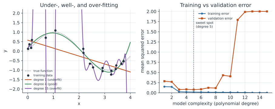
The left panel of the figure tells the whole story. A model that is too simple — the straight line — cannot capture the real pattern; it underfits, making systematic errors no matter how much data it sees. A model that is too flexible — the degree-15 polynomial — bends to pass near every point, capturing the noise as if it were signal; it overfits, and its wild wiggles are disastrous between the training points. The middle model is about right. The formal statement is the bias–variance decomposition: for squared-error loss, the expected error on a new point splits into three pieces, $$\mathbb{E}\!\left[(y - \hat f(x))^2\right] = \underbrace{\left(\mathbb{E}[\hat f(x)] - f(x)\right)^2}_{\text{bias}^2} + \underbrace{\mathbb{E}\!\left[(\hat f(x) - \mathbb{E}[\hat f(x)])^2\right]}_{\text{variance}} + \underbrace{\sigma^2}_{\text{irreducible}}, \tag{1}$$ where bias is how far the model’s average prediction is from the truth, variance is how much the fit jumps around as the training set changes, and $\sigma^2$ is noise no model can remove. Simple models are high-bias, low-variance; flexible models are low-bias, high-variance; and the decomposition (1) says the best model trades one against the other rather than minimizing either alone.

Training error lies: the validation set#

The right panel shows why you cannot trust training error. As complexity grows, training error falls monotonically — a flexible enough model can drive it to zero by memorizing — so the model that looks best on its own training data is precisely the one that has overfit. What you actually care about is error on data the model has not seen, estimated by holding out a validation set before fitting. Validation error is U-shaped: it falls as the model stops underfitting, bottoms out at the sweet spot, then rises as overfitting sets in, and the gap between the training and validation curves is the overfitting. The standard discipline uses three splits: a training set to fit parameters, a validation set to choose the model and its complexity, and a test set touched exactly once, at the very end, to report honest performance. The test set is sacred — reuse it to make choices and it quietly becomes a validation set, and your reported accuracy becomes a lie.

Cross-validation#

Holding out a single validation set wastes data and makes the estimate noisy, which hurts when data are scarce. $k$-fold cross-validation fixes both: split the data into $k$ equal folds, then train $k$ times, each time holding out a different fold for validation and averaging the $k$ scores. Every point is used for validation exactly once and for training $k-1$ times, so the estimate uses all the data and is far more stable. Common choices are $k=5$ or $k=10$; the extreme $k=n$ is leave-one-out cross-validation. For time series the folds must respect time — you validate on the future, never train on data that comes after your validation point — or you leak information and flatter yourself.

Regularization#

Rather than limit a model’s flexibility by hand, regularization lets it be flexible but penalizes complexity, adding a term to the loss that pulls the parameters toward zero: $$\hat\theta = \arg\min_\theta \Bigl[\, \underbrace{\mathcal{L}(\theta)}_{\text{fit}} + \lambda\, \underbrace{R(\theta)}_{\text{penalty}} \Bigr].$$ The strength $\lambda$ is a hyperparameter chosen by cross-validation, and it slides the model along the bias–variance curve: $\lambda=0$ is the unregularized (overfitting-prone) fit, large $\lambda$ forces a simple one. The two classic penalties differ in a consequential way. Ridge ($L_2$) regularization uses $R(\theta)=\sum_j \theta_j^2$, shrinking all coefficients smoothly toward zero and taming variance. Lasso ($L_1$) uses $R(\theta)=\sum_j |\theta_j|$, which drives some coefficients exactly to zero, performing automatic variable selection — valuable when you suspect only a few of many predictors matter. For neural networks the same idea appears as weight decay ($L_2$ on the weights), dropout (randomly zeroing units during training so the network cannot rely on any one), and early stopping (halting training when validation error starts to rise) — the mechanism the LSTM and CNN pages quietly depend on.

A worked example#

Fit polynomials of increasing degree to $30$ noisy points from $f(x)=\sin(1.5x)$, scoring each by 5-fold cross-validation. The degree-1 fit has high CV error (underfit); the error falls to a minimum around degree 4–5, then climbs steeply as the high-degree fits overfit and their cross-validated error explodes even as their training error keeps shrinking. Take the degree-15 model — badly overfit on its own — and add ridge regularization: a modest penalty reins in the wild coefficients and pulls the cross-validated error back down toward the well-chosen low-degree model, while too large a penalty over-shrinks and underfits again — the same U-shape, now in the penalty strength $\lambda$. The lesson is that complexity is not the enemy; unregularized, unvalidated complexity is.

In code#

Python#

Cross-validation makes the U-shaped curve concrete — training error falls with degree while cross-validated error turns back up:

import numpy as np
from sklearn.pipeline import make_pipeline
from sklearn.preprocessing import PolynomialFeatures, StandardScaler
from sklearn.linear_model import LinearRegression, Ridge
from sklearn.model_selection import cross_val_score, KFold

rng = np.random.default_rng(0)
X = np.sort(rng.uniform(0, 4, 30))[:, None]
y = np.sin(1.5 * X.ravel()) + rng.normal(0, 0.25, 30)
kf = KFold(5, shuffle=True, random_state=0)

for deg in (1, 4, 15):
    model = make_pipeline(PolynomialFeatures(deg), StandardScaler(), LinearRegression())
    cv = -cross_val_score(model, X, y, cv=kf,
                          scoring="neg_mean_squared_error").mean()
    train = np.mean((model.fit(X, y).predict(X) - y) ** 2)
    print(f"degree {deg:2d}:  train MSE {train:.3f}   5-fold CV MSE {cv:.3f}")

degree  1:  train MSE 0.218   5-fold CV MSE 0.256
degree  4:  train MSE 0.042   5-fold CV MSE 0.058
degree 15:  train MSE 0.033   5-fold CV MSE 0.094

Regularization lets the over-flexible degree-15 model recover — a modest ridge penalty pulls its cross-validated error back down toward the sweet spot, while too large a penalty over-shrinks and underfits again:

for alpha in (0.0, 1e-2, 1.0):
    est = Ridge(alpha=alpha) if alpha else LinearRegression()
    model = make_pipeline(PolynomialFeatures(15), StandardScaler(), est)
    cv = -cross_val_score(model, X, y, cv=kf,
                          scoring="neg_mean_squared_error").mean()
    print(f"degree 15, ridge alpha={alpha:<5}: 5-fold CV MSE {cv:.3f}")

degree 15, ridge alpha=0.0  : 5-fold CV MSE 0.094
degree 15, ridge alpha=0.01 : 5-fold CV MSE 0.065
degree 15, ridge alpha=1.0  : 5-fold CV MSE 0.153

R#

# caret / glmnet handle cross-validation and L1/L2 regularization directly.
library(glmnet)
# cv.glmnet does k-fold CV over the penalty lambda automatically:
fit <- cv.glmnet(x = model.matrix(~ poly(x, 15), df), y = df$y, alpha = 0)  # ridge
fit$lambda.min                     # the CV-optimal penalty
coef(fit, s = "lambda.min")        # shrunken coefficients

Julia#

# MLJ provides resampling (CV) and tunable regularized models.
using MLJ
model = (@load RidgeRegressor pkg=MLJLinearModels)()
cv = CV(nfolds = 5, shuffle = true)
evaluate(model, X, y, resampling = cv, measure = rms)   # cross-validated RMSE

Why it matters#

Overfitting is the failure mode behind most machine-learning disappointments in epidemiology and public health. A risk score that looked stellar in development but collapses in a new hospital, an outbreak forecaster that nailed the past but missed the next wave, a diagnostic image classifier that keyed on a scanner artefact — all are overfitting, dressed up. The defenses are unglamorous and non-negotiable: hold out a true test set, cross-validate every modelling choice, regularize flexible models, and — the strongest test of all — validate externally, on data from a different time, place, or population than the model was built on. This discipline is what separates a model that describes its training data from one that can be trusted on the next patient, the next county, and the next season.

Related#

• Neural Networks and the Multilayer Perceptron
• Linear Regression
• Bayesian Inference
• Hierarchical (Multilevel) Models
• Maximum Likelihood Estimation
• Convolutional Networks and Image Identification
• Proper Scoring Rules
• Quantitative Methods