Variational Autoencoders

An autoencoder learns to compress data through a narrow bottleneck and rebuild it, so the bottleneck is forced to keep only what matters. A variational autoencoder (VAE) makes that bottleneck probabilistic: instead of a single code it learns a small cloud of plausible codes for each input, regularized so the whole latent space is smooth and continuous. That upgrade turns the autoencoder into a proper generative model you can sample from, and it gives a principled anomaly score — how badly the model reconstructs an input — which is why VAEs show up in surveillance, genomics, and as a way to encode complex priors for Bayesian computation.

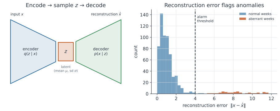
Encoder, decoder, and the latent space#

A VAE has two neural networks trained together. The encoder $q_\phi(\mathbf{z}\mid\mathbf{x})$ maps an input $\mathbf{x}$ to a distribution over a low-dimensional latent vector $\mathbf{z}$ — concretely it outputs a mean $\boldsymbol{\mu}(\mathbf{x})$ and a standard deviation $\boldsymbol{\sigma}(\mathbf{x})$, defining a Gaussian $\mathcal{N}(\boldsymbol{\mu}, \operatorname{diag}\boldsymbol{\sigma}^2)$. The decoder $p_\theta(\mathbf{x}\mid\mathbf{z})$ maps a latent vector back to a reconstruction of the input. A prior $p(\mathbf{z}) = \mathcal{N}(\mathbf{0}, I)$ says what codes are plausible before seeing any data. The latent dimension is deliberately much smaller than the input, so the network cannot simply memorize — it must discover a compact set of factors (a “seasonal level”, a “case-mix”) that explain the data.

The objective: the ELBO#

We would like to maximize the likelihood $p_\theta(\mathbf{x}) = \int p_\theta(\mathbf{x}\mid\mathbf{z})\,p(\mathbf{z})\,d\mathbf{z}$, but that integral is intractable. Variational inference replaces it with a tractable lower bound, the evidence lower bound (ELBO): $$\log p_\theta(\mathbf{x}) \;\ge\; \underbrace{\mathbb{E}_{q_\phi(\mathbf{z}\mid\mathbf{x})}\!\left[\log p_\theta(\mathbf{x}\mid\mathbf{z})\right]}_{\text{reconstruction}} \;-\; \underbrace{D_{\mathrm{KL}}\!\left(q_\phi(\mathbf{z}\mid\mathbf{x}) \,\|\, p(\mathbf{z})\right)}_{\text{regularizer}}. \tag{1}$$ The two terms pull against each other and that tension is the whole design. The reconstruction term rewards codes that let the decoder rebuild the input faithfully. The KL term — a Kullback–Leibler divergence — penalizes the encoder for straying from the prior, pulling every input’s latent cloud toward $\mathcal{N}(\mathbf{0}, I)$; this is what keeps the latent space smooth and gap-free, so that nearby codes decode to similar outputs and you can interpolate or sample. For diagonal Gaussians the KL term is closed-form, $$D_{\mathrm{KL}}\!\left(\mathcal{N}(\boldsymbol{\mu}, \boldsymbol{\sigma}^2)\,\|\,\mathcal{N}(\mathbf{0}, I)\right) = \tfrac12 \sum_{j}\left(\mu_j^2 + \sigma_j^2 - \log \sigma_j^2 - 1\right),$$ so only the reconstruction term needs sampling.

The reparameterization trick#

To train by gradient descent we must backpropagate through the random sampling of $\mathbf{z}\sim\mathcal{N}(\boldsymbol{\mu},\boldsymbol{\sigma}^2)$, but you cannot differentiate through a raw random draw. The reparameterization trick moves the randomness out of the way: draw a standard normal $\boldsymbol{\varepsilon}\sim\mathcal{N}(\mathbf{0}, I)$ and set $$\mathbf{z} = \boldsymbol{\mu} + \boldsymbol{\sigma}\odot\boldsymbol{\varepsilon}.$$ Now $\mathbf{z}$ is a deterministic, differentiable function of the encoder outputs $\boldsymbol{\mu}, \boldsymbol{\sigma}$, with all the noise isolated in $\boldsymbol{\varepsilon}$, so gradients flow to the encoder and the ELBO can be optimized end to end.

Anomaly detection from reconstruction error#

A VAE trained on “normal” data learns to reconstruct it well. Feed it something unlike anything in training — an aberrant surveillance week, a corrupted image, a novel genome — and the decoder rebuilds it badly, so the reconstruction error $\lVert\mathbf{x} - \hat{\mathbf{x}}\rVert$ spikes. Thresholding that error, as on the right of the figure, gives an unsupervised anomaly detector that needs no labelled outbreaks, only examples of business-as-usual. This is a learned, multivariate cousin of the aberration-detection algorithms used in routine surveillance.

A worked example#

Take a one-dimensional latent with encoder output $\mu = 1.5$ and $\sigma = 0.5$ for some input. The KL penalty for this code is $\tfrac12(\mu^2 + \sigma^2 - \log\sigma^2 - 1) = \tfrac12(2.25 + 0.25 - \log 0.25 - 1) = \tfrac12(1.5 + 1.386) = 1.44$ nats, the price paid for placing the code away from the prior mean. To sample a latent, draw $\varepsilon = 0.4$ and set $z = 1.5 + 0.5\times 0.4 = 1.7$; the decoder turns $z = 1.7$ into a reconstruction. Because the trick writes $z$ as $\mu + \sigma\varepsilon$, the derivatives $\partial z/\partial\mu = 1$ and $\partial z/\partial\sigma = \varepsilon = 0.4$ are available, so training can adjust $\mu$ and $\sigma$ to improve the reconstruction.

In code#

Python#

A linear autoencoder is exactly principal component analysis, so we can demonstrate the reconstruction-error anomaly detector — the practical payoff of a VAE — with a runnable PCA stand-in, then show the full probabilistic VAE illustratively.

import numpy as np
from sklearn.decomposition import PCA
rng = np.random.default_rng(0)

# "normal" weeks: 20-dim syndromic profiles living near a 3-factor subspace
factors = rng.standard_normal((300, 3))
loading = rng.standard_normal((3, 20))
X = factors @ loading + 0.3 * rng.standard_normal((300, 20))

ae = PCA(n_components=3, svd_solver="full").fit(X)      # linear autoencoder
recon = ae.inverse_transform(ae.transform(X))           # encode then decode
err = np.sqrt(((X - recon) ** 2).sum(1))                # reconstruction error
thr = err.mean() + 3 * err.std()                        # alarm threshold

aberrant = (rng.standard_normal((3, 20)) * 4).clip(-6, 6)  # weeks off the manifold
aberr_err = np.sqrt(((aberrant - ae.inverse_transform(ae.transform(aberrant))) ** 2).sum(1))
print(f"normal error: mean {err.mean():.2f}, 99th pct {np.percentile(err, 99):.2f}")
print(f"threshold: {thr:.2f}")
print("aberrant week errors:", np.round(aberr_err, 1), "-> all flagged:",
      bool(np.all(aberr_err > thr)))

normal error: mean 1.22, 99th pct 1.69
threshold: 1.82
aberrant week errors: [17.3 15.5 14.9] -> all flagged: True

The reparameterization trick and the ELBO are short enough to see directly:

def kl_standard_normal(mu, sigma):
    return 0.5 * np.sum(mu ** 2 + sigma ** 2 - np.log(sigma ** 2) - 1)

mu, sigma = np.array([1.5]), np.array([0.5])
eps = rng.standard_normal(mu.shape)          # noise, outside the gradient path
z = mu + sigma * eps                         # reparameterized latent sample
print(f"KL penalty {kl_standard_normal(mu, sigma):.3f} nats;  z sample {z[0]:.3f}")

KL penalty 1.443 nats;  z sample 2.437

The full nonlinear VAE trains in PyTorch on the same syndromic data, and its reconstruction error separates normal from aberrant weeks just as the linear stand-in did — but with a nonlinear encoder and decoder and the true ELBO as the loss:

import torch, torch.nn as nn
torch.manual_seed(0)
Xt = torch.tensor(X, dtype=torch.float32)          # the 20-dim weeks from above

class VAE(nn.Module):
    def __init__(self, d_in=20, d_lat=3):
        super().__init__()
        self.enc = nn.Linear(d_in, 2 * d_lat)      # outputs mu and log-variance
        self.dec = nn.Sequential(nn.Linear(d_lat, 32), nn.ReLU(), nn.Linear(32, d_in))

    def forward(self, x):
        mu, logvar = self.enc(x).chunk(2, dim=-1)
        z = mu + torch.exp(0.5 * logvar) * torch.randn_like(mu)   # reparameterize
        return self.dec(z), mu, logvar

vae = VAE()
opt = torch.optim.Adam(vae.parameters(), lr=0.01)
for epoch in range(400):
    opt.zero_grad()
    xhat, mu, logvar = vae(Xt)
    recon = nn.functional.mse_loss(xhat, Xt, reduction="sum")
    kl = -0.5 * torch.sum(1 + logvar - mu ** 2 - logvar.exp())
    (recon + kl).backward()                        # minimize the negative ELBO
    opt.step()

with torch.no_grad():                              # score by decoding the latent mean
    def recon_err(x):
        mu, _ = vae.enc(x).chunk(2, dim=-1)
        return (vae.dec(mu) - x).pow(2).sum(1).sqrt()
    en = recon_err(Xt).mean().item()
    ea = recon_err(torch.tensor(aberrant, dtype=torch.float32)).mean().item()
print(f"mean reconstruction error  normal {en:.1f}  aberrant {ea:.1f}")
print(f"aberrant weeks flagged (error > 3x normal): {ea > 3 * en}")

mean reconstruction error  normal 1.3  aberrant 15.9
aberrant weeks flagged (error > 3x normal): True

R#

# torch for R; here the encoder/decoder skeleton of a VAE.
library(torch)
vae <- nn_module(
  initialize = function(d_in, d_lat) {
    self$enc <- nn_linear(d_in, 2 * d_lat)       # mu and log-variance
    self$dec <- nn_linear(d_lat, d_in)
  },
  forward = function(x) {
    ms <- self$enc(x); d <- ncol(ms) / 2
    mu <- ms[, 1:d]; logvar <- ms[, (d + 1):(2 * d)]
    z <- mu + torch_exp(0.5 * logvar) * torch_randn_like(mu)
    list(self$dec(z), mu, logvar)
  }
)

Julia#

# Flux with an explicit reparameterized sampling step.
using Flux
enc = Dense(20 => 6)          # -> [mu; logvar], 3 latent dims
dec = Chain(Dense(3 => 64, relu), Dense(64 => 20))
function reparam(mu, logvar)
    mu .+ exp.(0.5f0 .* logvar) .* randn(Float32, size(mu))
end

Why it matters#

The VAE’s two gifts — a smooth low-dimensional representation and a reconstruction-based anomaly score — both map onto epidemiology. As an anomaly detector it learns the shape of normal surveillance data and flags departures without needing labelled outbreaks, complementing classical aberration detection. As a representation learner it compresses high-dimensional data — pathogen genomes, cytometry panels, serological profiles — into a few interpretable latent axes for clustering and visualization. As a generative model it can produce synthetic-but-realistic records that share the statistics of sensitive health data without copying any individual, a route to privacy-preserving data sharing. And, most distinctively for this field, a VAE can encode a complex prior: train it to reproduce draws from a spatial or mechanistic prior, then reuse its decoder to make otherwise-intractable Bayesian spatial inference fast — the subject of the next page.

Related#

• Encoding Spatial Priors with VAEs (PriorVAE)
• Kullback–Leibler Divergence
• Neural Networks and the Multilayer Perceptron
• Bayesian Inference
• Aberration Detection
• Gaussian Processes
• Recurrent Networks and LSTMs
• Deep Learning, Foundation Models, and Agentic AI
• Quantitative Methods